Understanding Quantum Boltzmann Machines

Generative models are everywhere in machine learning, but physicists had a working generative model more than a century before anyone talked about GANs or diffusion: the Boltzmann distribution. Give me an energy function and a temperature, and I can hand you a recipe for sampling configurations of a physical system. In this post I want to walk through [1], Learning to generate high-dimensional distributions with low-dimensional quantum Boltzmann machines, which asks a very physics-flavoured question about quantum machine learning: if you upgrade a classical Boltzmann machine to a quantum Boltzmann machine (QBM), does a small quantum model get access to correlations that its wiring diagram alone shouldn't allow?

The answer is yes, and the mechanism — non-commuting operators smuggling correlations across qubits that were never directly coupled — is worth understanding slowly, the way you'd explain it to a student seeing it for the first time.

From spins to samples: what is a Boltzmann machine?

Start classical. A Boltzmann machine (BM) describes a bit string $s = s_0 s_1 \cdots s_{n-1}$, $s_i \in \{-1,+1\}$, through an energy function $E(s)$ and the associated Gibbs distribution

If you've read my earlier post on the Ising model, this should look familiar — it's exactly an Ising-type Hamiltonian [2], generalised to have a free weight on every site and every allowed interaction:

Every bit is a visible unit here — you observe it directly, as opposed to hidden units that only exist to help the model represent correlations it otherwise couldn't. A fully-visible BM is the simplest possible generative model: no hidden units, just an energy function over the data itself. The catch is expressivity. If your energy function only contains nearest-neighbour terms $s_i s_{i+1}$, the model can only ever represent correlations that respect that same nearest-neighbour graph. Reach for anything more structured — three-body correlations, correlations between distant sites — and a fully-visible classical BM simply cannot get there without adding hidden units, which is exactly why restricted Boltzmann machines (RBMs) became the practical default, at the cost of an intractable partition function for anything but small systems.

Making it quantum

A quantum Boltzmann machine keeps the same skeleton — a parametrised Hamiltonian, a Gibbs state, a temperature — but the energy function becomes a genuine quantum operator built from Pauli strings:

where each $H_i$ is a one- or two-body Pauli string ($Z_i$, $Z_iZ_j$, but also $X_i$, $X_iY_j$, and so on) and $\rho_\theta$ is now a density matrix rather than a diagonal probability vector. If you restrict $H_\theta$ to only $Z$ and $ZZ$ terms, $\rho_\theta$ stays diagonal in the computational basis and you recover an ordinary classical BM exactly. The entire generalisation — and everything interesting that follows — comes from allowing terms that don't commute with each other.

That single change matters more than it sounds like it should. A classical spin is a switch: it points up or down, and correlating two switches requires an explicit wire between them. A qubit is not a switch — it lives in a superposition, and two qubits coupled through non-commuting operators can end up correlated even along a path where there is no direct term in the Hamiltonian at all:

This is the entire thesis of the paper, stated as a picture in its own Figure 1:

The authors define the dimension of a distribution as the dimension of the lattice needed to generate it classically: a chain is one-dimensional, a grid is two-dimensional, all-to-all connectivity is $(n-1)$-dimensional. Their central claim is that a low-dimensional QBM — one whose Hamiltonian only has nearest-neighbour terms — can learn distributions of higher dimension than its own connectivity graph. Classically that would require either more edges or hidden units; quantum mechanically, entanglement does the work for free.

You can make this precise with conditional mutual information. For subsystems $A$, $B$, $C$ of a state $\rho$,

where $S(\cdot)$ is the von Neumann entropy. For a classical nearest-neighbour chain this vanishes exactly whenever $B$ separates $A$ from $C$ — that's just the Markov property of a 1D classical chain. The paper shows numerically that a nearest-neighbour-connected QBM has non-zero $\mathcal{I}(0\!:\!2\,|\,1)$ even though qubits 0 and 2 share no term in $H_\theta$: correlation is leaking through the middle qubit via entanglement, not via an explicit coupling.

Training: same recipe, different bookkeeping

Training a QBM looks almost identical to training a classical BM. You minimise the quantum relative entropy between a target state $\eta$ (your data, embedded as a density matrix) and the model state $\rho_\theta$:

For a classical BM this reduces exactly to the ordinary KL divergence between $p(s)$ and $q_\theta(s)$. The gradient with respect to each Hamiltonian weight has the same contrastive-divergence flavour you'd expect from a classical BM:

the difference between the expectation value of $H_i$ on the data and on the model. Nothing about this formula requires $H_i$ to commute with anything else — it is the one line of the classical training rule that silently generalises to the full quantum case. The practical headache is that preparing $\rho_\theta$ exactly requires diagonalising a non-diagonal Gibbs state, which gets expensive fast; the paper works around this with thermal pure quantum (TPQ) states, a statistical trick for estimating $\mathrm{Tr}(\rho_\theta H_i)$ from a handful of pseudo-random pure states rather than the full density matrix. It's a computational detail rather than a conceptual one, so I won't dwell on it — the important part is that the loss and its gradient are exactly the classical BM recipe, evaluated on a genuinely quantum object.

Does the extra machinery pay off?

The first test is entirely synthetic: four qubits, all-to-all connectivity, both a BM and a QBM equipped with a generic Hamiltonian (all one- and two-body Pauli strings), trained on 1000 randomly generated three-body Boltzmann distributions.

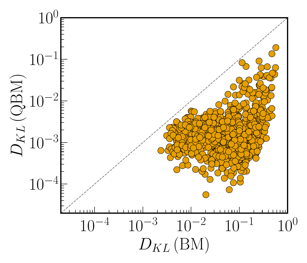
The comparison is deliberately fair: both models have up to two-body interactions and the same connectivity graph. The gap in performance isn't coming from extra parameters, it's coming from the fact that the target distributions contain genuine three-body correlations, which a two-body classical energy function cannot represent no matter how you tune the weights — while the QBM's non-commuting two-body Pauli terms can fake a three-body effect through entanglement.

A real target: particle jets

Synthetic Boltzmann distributions are a clean testbed, but the paper's more interesting experiment uses real collider data. A jet is a collimated spray of particles produced when a quark or gluon fragments and hadronizes; the momentum shared between the leading particles inside a jet is highly correlated by construction — it has to add up to the jet's total momentum, and QCD radiation patterns leave characteristic correlations behind. Using the JetNet dataset, the authors build a joint probability distribution over the (binned) relative transverse momentum $|p_T^{\rm rel}|$ of the four hardest particles in a jet:

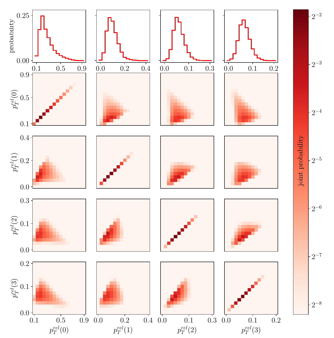
Discretising four particles into 16 bins each needs 16 qubits — small enough to simulate, large enough to be a genuine stress test. Training both BMs and QBMs (with all-to-all connectivity) across system sizes from 4 to 16 qubits, for both $m=2$ and $m=4$ particle datasets, gives the headline result:

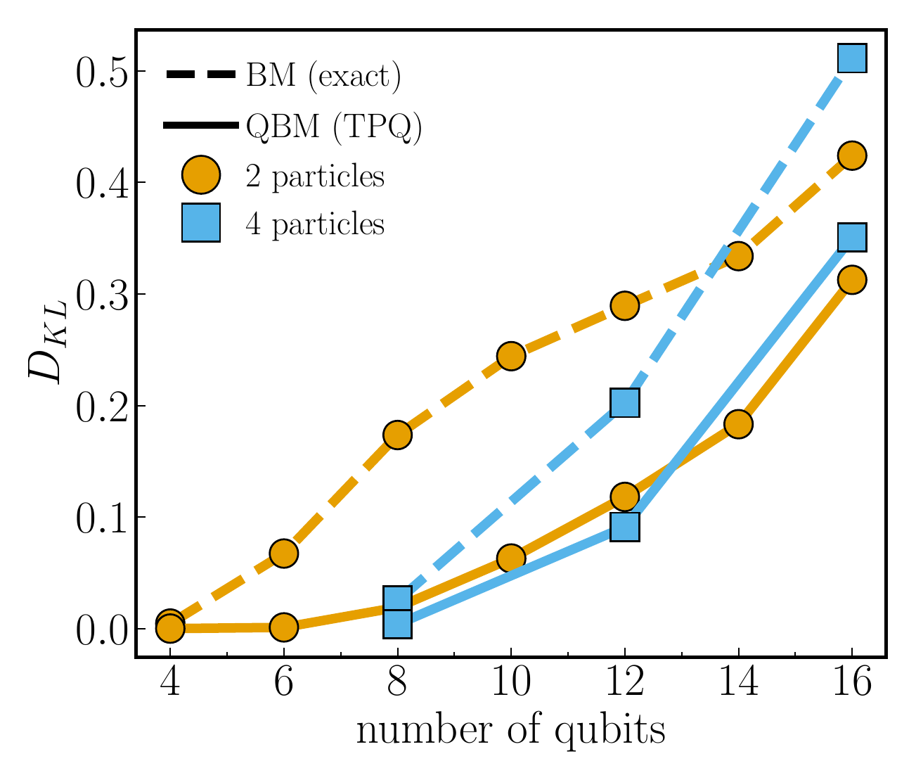
Perhaps the most striking follow-up result — not reproduced here, but worth stating — is that a QBM restricted to nearest-neighbour-particle connectivity (units within a particle fully connected, particles chained to their neighbours by $|p_T^{\rm rel}|$ ordering) can match an all-to-all connected classical BM. The quantum model with a sparser wiring diagram ties the classical model with a denser one. That's the practical payoff of the entanglement argument from the previous section: you don't need to pay for all-to-all connectivity if non-commuting terms can smuggle the correlation through for you.

Where this leaves us

None of this is a free lunch. QBM training is expensive precisely because Gibbs states of non-commuting Hamiltonians can't be classically simulated the easy way a diagonal BM can — the TPQ/Lanczos machinery exists to work around that cost, and it introduces its own finite-size systematic error. The system sizes tested here top out at 16 qubits on a classical simulator; a genuine quantum-hardware advantage would need fault-tolerant devices with far more logical qubits than exist today. What the paper does establish convincingly is the mechanism: non-commuting Hamiltonian terms are not a nuisance to be minimised, they are the entire source of a fully-visible QBM's extra representational power over its classical counterpart, and that power shows up on a genuine, correlated, high-energy-physics dataset and not just on constructed toy examples.

I like this line of work for the same reason I liked writing about a physics-informed quantum circuit for QCD splittings: the interesting question in near-term quantum machine learning for particle physics is rarely "can a big enough quantum circuit fit this data" — it's "does the quantum structure buy you something a classical model of the same size provably cannot have." Here the answer is entanglement standing in for connectivity, and it holds up on real jet data.

References